NURBS Curves: How to use Knot Vectors

When working in Maya, we create curves freely without crunching numbers. We use them in Maya Hair, Spline IK rigs, Motion/Flow paths, as control curves for characters rigs, create them procedurally for modeling, amongst other uses. My goal in this post is for you to better understand how to generate curves using knot vectors.

---

Linear curves are simply lines that follow the standard y = mx + b formula. In Maya, they are created as a curve of 1 degree. That means that the highest power in the equation is 1. In theory, this curve type has 2 knots. The relation between knots to CV is: #knots = (#CVs+deg -1).

string $curve = `curve -d 1 -p -2 0 0 -p 2 0 -2`;

Simply pass in your two points, and tell Maya that you’re drawing a linear curve. Let’s attach a curveInfo node to this curve and poke around a little bit.

string $cInfo = `arclen -ch 1 $curve`;
getAttr($cInfo+".knots[*]");
// Result: 0 1 //
 
It seems that there are two knots on this curve that are weighted to each CV on the curve. Using #knots = (#CVs+deg -1), we know that we have 2 CVs on a curve of 1 degree, minus 1: that’s 2 knots. So we know that checks out.

Before we investigate further, let’s try the same thing with a quadratic curve. Behind the scenes, Maya will draw the smooth curve using an equation where the highest degree order is 2. Since we all miss our high school math classes, let’s draw a parabola:

$curve = `curve -d 2 -p -1 0 -2 -p -1 0 0 -p 1 0 0 -p 1 0 -2`;
$cInfo = `arclen -ch 1 $curve`;
getAttr($cInfo+".knots[*]");
// Result: 0 0 1 2 2 //
 
We have a curve of 2 degrees, we plotted 4 points, minus 1: that’s a total of 5 knots. The collection of knots on a curve is referred to its Knot Vector. However, what do these knot magnitudes mean? Each element in the vector determines where in parameter space the curve will be drawn. I know that’s a very vague statement but please stay with me!

Think of the first and last points on a curve as an anchor. This is the most common type of knot vector: Pinned Uniform Knot Vectors. Each anchor needs to be held down by the same number of knots as the curve’s degree. In our first example, we had a curve of 1 degree being pinned down by one knot on each end point. In our second example, we had a curve being held down by 2 knots on each end point.

So then what does the 1 mean in the [0 0 1 2 2] result? It turns out that these numbers are arbitrary. The number values don’t matter in a Knot Vector. Say what? Yes, that’s right. What matters is the ratios of the values to each other. The main rule is that Maya requires each knot’s magnitude to be in ascending order. So what happens if we create a curve but mess with that middle knot? What results will we get? Let’s try it!

curve -d 2 -p -1 0 -2 -p -1 0 0 -p 1 0 0 -p 1 0 –2
      -k 0 -k 0 -k 0 -k 2 -k 2;

By specifying the knot values to the curve command, it seems we have created a curve with non-uniform weighting. We modified the middle knot in a way that we made the curve appear discontinuous.

Just for fun, we can weight the center knot to the other end to get a mirrored result.

curve -d 2 -p -1 0 -2 -p -1 0 0 -p 1 0 0 -p 1 0 –2
      -k 0 -k 0 -k 2 -k 2 -k 2;

Go ahead and release the pins on this 2nd degree curve. Notice that you can easily un-anchor the curve from their start and end points by simply supplying different weights. This also makes your curve a lot shorter. This is something you need to try for yourself because it’s one of those things that are too abstract in words.

Uniformly distributing our knots makes our NURBS curve simply a B-Spline. Having the ability to specify and interactively adjust the knots is a feature of NURBS, or Non-Uniform Rational B-Splines. Allowing a partial knot weight is a nice feature:

curve -d 2 -p -1 0 -2 -p -1 0 0 -p 1 0 0 -p 1 0 –2
      -k 0 -k 0 -k 1.5 -k 2 -k 2;
curve -d 2 -p -1 0 -2 -p -1 0 0 -p 1 0 0 -p 1 0 –2
      -k 0 -k 0 -k 0.5 -k 2 -k 2;

Finally, to nail the point, let’s try drawing an pinned cubic curve with a degree of 3.

curve -d 3 -p -1 0 -3 -p -2 0 -2 -p 0 0 0 -p 2 0 -2 -p 1 0 –3
      -k 0 -k 0 -k 0 -k 1 -k 2 -k 2 -k 2;

Notice that I used 3 pinned knots to hold down the end points. The middle knot is exactly half way between 0 and 2. This makes the curve uniformly weighted. If you have questions, please let me know in the comment section! I’m sure there are things I can clarify. I want to be sure the information comes through clearly.

---

Notes:
- Maya seems to ignore knot magnitudes on linear curves.
- When creating curves with the -pointWeight flag, accurate knot values are not returned.
- When editing curves created with the -pointWeight flag in the viewport, the curves seem to snap to a weighted value of 1 to each CV.

A List of My Favorite Books

Several people have asked me about what resources I use to learn my favorite topics. There are informative videos and written tutorials scattered all over the web, and only but a few are concise, efficient, and well prepared. This is why I rely mostly on books that are written by seasoned professionals that know a thing or two about teaching. Here is a list of the books I am in love with:

• MEL Scripting for Maya Animators
• Mastering Autodesk Maya
• Stop Staring: Facial Modeling and Animation Done Right
• Maya Python for Games and Film
• Complete Maya Programming I & II
• Art of Rigging I & II
• Professional MEL Solutions for Production
• Maya Visual Effects: The Innovator's Guide
• 3D Math Primer for Graphics and Game Development
• Game Development with ActionScript

These gems are not listed in any particular order but MEL Scripting for Maya Animators was the first book I ever read on MEL, or Maya for that matter. I bought the very first edition of that text because I was looking for a source of inspiration when I was stuck at home writing Game Development with ActionScript. They are both considered oldies as far as technology goes, so they might be tough to find.

Understanding 3D Vectors

DISCLAIMER: This post covers the vector type in Maya. If you are new to vectors, please acquaint yourself with them and review the help docs before reading this post. I tried to keep this post as light on math as possible, however, I will clarify where needed, based on your suggestions. This is a huge topic and this post merely summarizes how useful vectors are.

User Guide > Scripting > MEL and Expressions > Useful functions

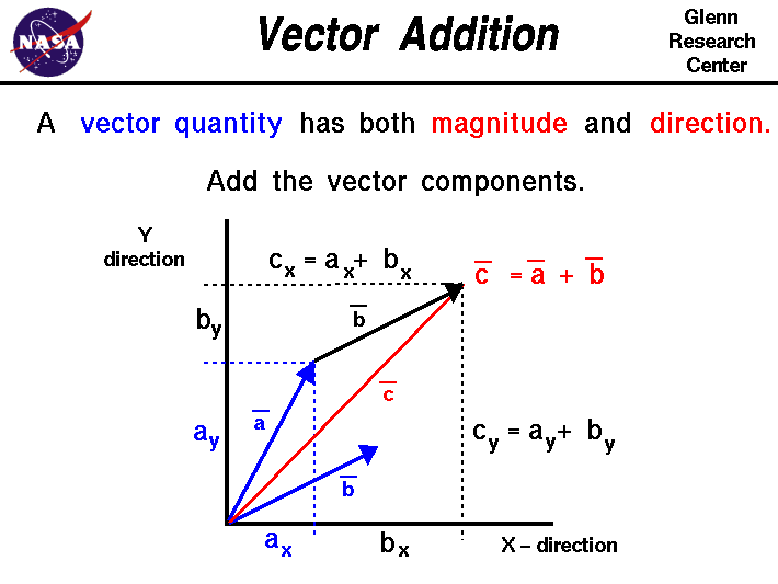
Let’s break one of our toys apart and learn how things work from the inside out. The knowledge we acquire from doing this allows us to build bigger and better toys. In physics, a vector is described as an entity that has both a magnitude and a direction. In MEL, a vector is represented by x, y, and z components. These components can be combined back into their scientific form at any time. Vectors can represent a location in space, the velocity and/or acceleration of an object, tracing rays between two points, etc.

Retrieving a vector’s magnitude is trivial in MEL:

vector $A = << 1, 2, 3>>;
vector $B = << 3, 2, 1>>;
int $length = mag($A);

Finding the direction vector can by done by using the unit function.

When you perform arithmetic with vectors, the output is considered the resultant. Addition yields a vector that is said to be a diagonal in a parallelogram.

This is interesting to us because if you were to take the B and move a copy (by adding it to A) to the head of A, we build ourselves a triangle that can used to solve for solutions. If we then move a copy of A to the head of B, we end up with a parallelogram. When you subtract a vector from another, the resultant yields a magnitude that is the distance between the heads of A and B. If you take B-A (, which is not the same as A-B, ) and add it to A, we have ourselves another triangle. Still with me? This is only possible because a vector can be equal (& parallel) to any other vector in space as long as they are equal in direction and magnitude. So if you need to reposition a vector, do so by adding it to another vector location. That was the heaviest paragraph in this post, I promise!

By multiplying a vector by a scalar value, we are simply scaling the the vector’s magnitude by that number. There are other types of vector products that are extremely important in computer graphics, the dot product, which yields a scalar value, and the cross product (, which yields another vector perpendicular to the first two. Nuff talk, let’s get to work.

---

In Maya, create 4 locators. Name them A, B, C, & D. In the script editor, retrieve their world space positions and store those values in vectors. Imagine each locator to be a ray, that originates at the origin, and each locator shape being the vector’s head. Spread the locators in space away from the origin and each other, arbitrarily and for variety.

Make C perpendicular to the first two, by taking the cross product of A & B and move C to the resultant. Now that you know that C perpendicular to the first two, there’s a good chance there is one axis that is not perpendicular to another. You can verify this by taking the dot product of two vectors. If the dot product is not 0, then your vectors are not perpendicular.

TIP: Make the result of AxC a unit vector, a vector with the length 1, by using the unit function on C. The 'x' in this notation signifies we're taking the cross product of these two vectors.

Anyway, take the cross product of A & C, and feed the result to B. You now have 3 axis that are perfectly orthogonal to each other. Assuming that A was already at the “lookAt” location, let’s place D along A’s axis, but with a magnitude of 1. Vectors of this length are called unit vectors. The process of getting this result is call normalization.

Normalize A and pipe the results right into D. You now have solved for the same things that the aim constraint solves for in most 3D software, including games. If you were to normalize all 3 orthogonal axes, you would have what is called an Orthonormal Basis.

Here's a code snippet:

// 3D (Basis) Vectors
// By Lewis M., 2013
// Usage:
// Arbitrarily place four locators in the scene
// Name them A, B, C, & D

// Retrieve A & B's locations
float $a_coord[] = `xform -q -ws -t A`;
float $b_coord[] = `xform -q -ws -t B`;

// Find an orthogonal vector to both A & B
vector $a = <<$a_coord[0], $a_coord[1], $a_coord[2]>>;
vector $b = <<$b_coord[0], $b_coord[1], $b_coord[2]>>;
vector $c = cross($a, $b);
vector $d;

// Scale it down to the length of 1
$c = unit($c);
move -a ($c.x) ($c.y) ($c.z) C;
print dot($a, $b); // Most likely not zero

// Adjust B to be orthogonal to both A and C
$b = cross($a, $c);
$b = unit($b);
move -a ($b.x) ($b.y) ($b.z) B;

// Finally, scale down A and place D in the position
$d = unit($a);
move -a ($d.x) ($d.y) ($d.z) D;

// Just for fun, draw some visually appealing curves
curve -d 1 -p 0 0 0 -p ($a.x) ($a.y) ($a.z) -k 0 -k 1 ;
curve -d 1 -p 0 0 0 -p ($b.x) ($b.y) ($b.z) -k 0 -k 1 ;
curve -d 1 -p 0 0 0 -p ($c.x) ($c.y) ($c.z) -k 0 -k 1 ;
//grid -tgl 0;
//refresh;

As an exercise, you can use MEL, Python, or even utility nodes to create the connections.



Above is a picture of my little aim constraint node setup.  It differs from my discussion above because this version is interactive. In this version, I am able to position A wherever I want and have the other locators automatically update. The NURBS curves you see there are strictly for visual appeal